window-function

window-function

Collection of window functions for signal processing and spectral analysis.

npm install window-function

import { hann, kaiser, generate, apply } from 'window-function'

// Every window: fn(i, N, ...params) → number
hann(50, 101)                    // single sample → 1.0

// Generate full window as Float64Array
let w = generate(hann, 1024)

// Apply window to a signal in-place
let signal = new Float64Array(1024).fill(1)
apply(signal, hann)              // signal *= hann

// Parameterized windows pass extra args
generate(kaiser, 1024, 8.6)     // Kaiser with β = 8.6

Or import individual windows directly:

import hann from 'window-function/hann'
import kaiser from 'window-function/kaiser'

Reference

Simple

rectangular · triangular · bartlett · welch · connes · hann · hamming · cosine · blackman · exactBlackman · nuttall · blackmanNuttall · blackmanHarris · flatTop · bartlettHann · lanczos · parzen · bohman

Parameterized

kaiser · gaussian · generalizedNormal · tukey · planckTaper · powerOfSine · exponential · hannPoisson · cauchy · rifeVincent · confinedGaussian

Array-computed

dolphChebyshev · taylor · kaiserBesselDerived · dpss · ultraspherical

Simple — no parameters

rectangular(i, N)

$w(n) = 1$

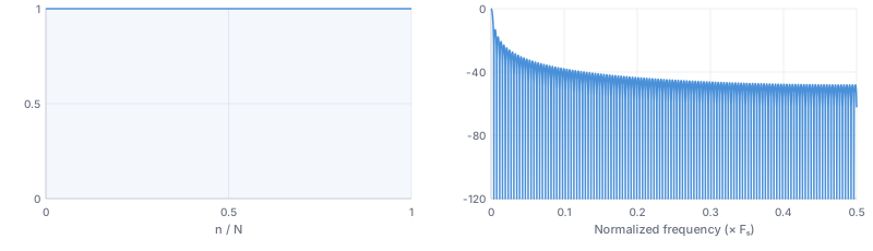
No windowing. Best frequency resolution, worst spectral leakage. Use for transient signals already zero at edges, or harmonic analysis with integer cycles. -13 dB sidelobe · -6 dB/oct rolloff

triangular(i, N)

$w(n) = 1 - \left|\frac{2n - N + 1}{N}\right|$

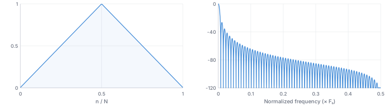
Linear taper, nonzero endpoints. Simple smoothing, 2nd-order B-spline. -27 dB sidelobe · -12 dB/oct rolloff

bartlett(i, N)

$w(n) = 1 - \left|\frac{2n - N + 1}{N - 1}\right|$

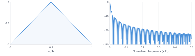
Linear taper, zero endpoints. Bartlett's method PSD estimation.[^bartlett1950] -27 dB sidelobe · -12 dB/oct rolloff

welch(i, N)

$w(n) = 1 - \left(\frac{2n - N + 1}{N - 1}\right)^2$

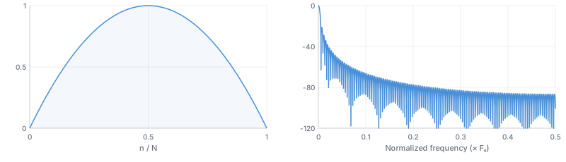
Parabolic taper. Welch's method PSD estimation.[^welch1967] -21 dB sidelobe · -12 dB/oct rolloff

connes(i, N)

$w(n) = \left[1 - \left(\frac{2n - N + 1}{N - 1}\right)^2\right]^2$

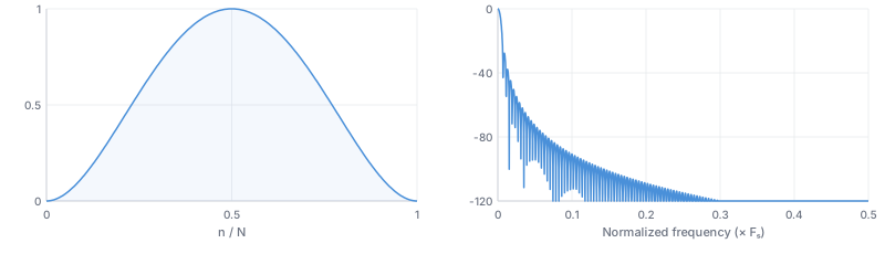
Welch squared (4th power parabolic). FTIR spectroscopy, interferogram apodization.[^connes1961] -24 dB/oct rolloff

hann(i, N)

$w(n) = 0.5 - 0.5\cos!\left(\frac{2\pi n}{N-1}\right)$

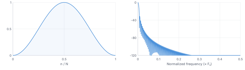
Raised cosine, zero endpoints. The default general-purpose choice. STFT with 50% overlap (COLA). Also called "Hanning" (misnomer).[^blackman1958] -32 dB sidelobe · -18 dB/oct rolloff

hamming(i, N)

$w(n) = 0.54 - 0.46\cos!\left(\frac{2\pi n}{N-1}\right)$

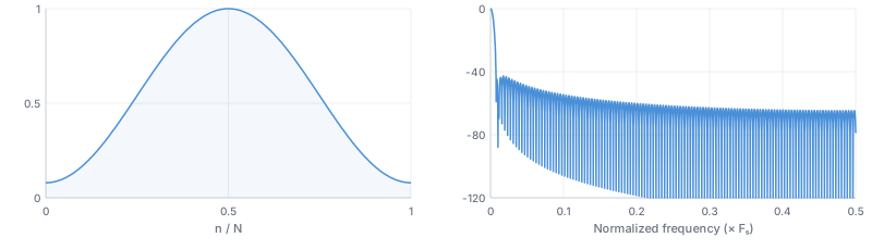
Raised cosine, nonzero endpoints. Optimized for first sidelobe cancellation. FIR filter design, speech processing.[^hamming1977] -43 dB sidelobe · -6 dB/oct rolloff

cosine(i, N)

$w(n) = \sin!\left(\frac{\pi n}{N-1}\right)$

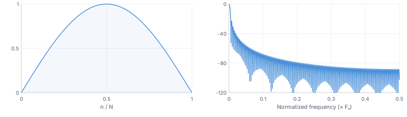
Half-period sine. MDCT audio codecs: MP3, AAC, Vorbis.[^princen1987] -23 dB sidelobe · -12 dB/oct rolloff

blackman(i, N)

$w(n) = 0.42 - 0.5\cos!\left(\frac{2\pi n}{N-1}\right) + 0.08\cos!\left(\frac{4\pi n}{N-1}\right)$

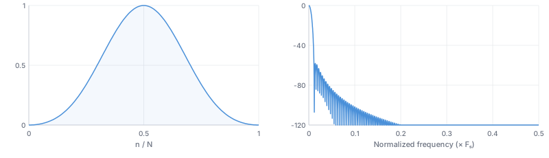
3-term cosine sum. Better leakage than Hann at the cost of wider main lobe.[^blackman1958] -58 dB sidelobe · -18 dB/oct rolloff

exactBlackman(i, N)

$w(n) = 0.42659 - 0.49656\cos!\left(\frac{2\pi n}{N-1}\right) + 0.076849\cos!\left(\frac{4\pi n}{N-1}\right)$

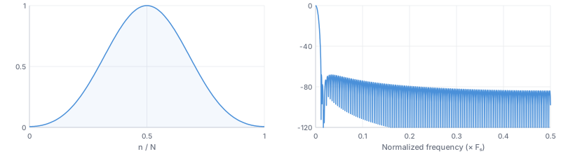
Blackman with exact zero placement at 3rd and 4th sidelobes.[^harris1978] -69 dB sidelobe · -6 dB/oct rolloff

nuttall(i, N)

$w(n) = 0.355768 - 0.487396\cos!\left(\frac{2\pi n}{N!-!1}\right) + 0.144232\cos!\left(\frac{4\pi n}{N!-!1}\right) - 0.012604\cos!\left(\frac{6\pi n}{N!-!1}\right)$

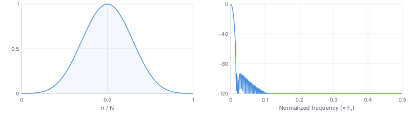
4-term cosine sum, continuous 1st derivative. High-dynamic-range analysis without edge discontinuity.[^nuttall1981] -93 dB sidelobe · -18 dB/oct rolloff

blackmanNuttall(i, N)

$w(n) = 0.3635819 - 0.4891775\cos!\left(\frac{2\pi n}{N!-!1}\right) + 0.1365995\cos!\left(\frac{4\pi n}{N!-!1}\right) - 0.0106411\cos!\left(\frac{6\pi n}{N!-!1}\right)$

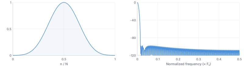
4-term cosine sum, lowest sidelobes among 4-term windows.[^nuttall1981] -98 dB sidelobe · -6 dB/oct rolloff

blackmanHarris(i, N)

$w(n) = 0.35875 - 0.48829\cos!\left(\frac{2\pi n}{N!-!1}\right) + 0.14128\cos!\left(\frac{4\pi n}{N!-!1}\right) - 0.01168\cos!\left(\frac{6\pi n}{N!-!1}\right)$

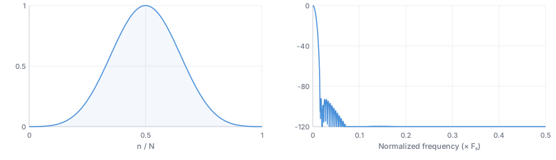
4-term minimum sidelobe. ADC testing, measurement instrumentation, >80 dB dynamic range.[^harris1978] -92 dB sidelobe · -6 dB/oct rolloff

flatTop(i, N)

$w(n) = 1 - 1.93\cos!\left(\frac{2\pi n}{N!-!1}\right) + 1.29\cos!\left(\frac{4\pi n}{N!-!1}\right) - 0.388\cos!\left(\frac{6\pi n}{N!-!1}\right) + 0.028\cos!\left(\frac{8\pi n}{N!-!1}\right)$

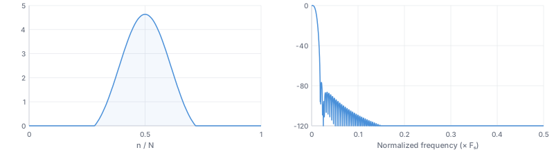
5-term cosine sum, near-zero scalloping. Peak ~4.64 (by design). Amplitude calibration, transducer calibration (~0.01 dB accuracy). ISO 18431.[^heinzel2002] -93 dB sidelobe · -6 dB/oct rolloff

bartlettHann(i, N)

$w(n) = 0.62 - 0.48\left|\frac{n}{N!-!1} - 0.5\right| - 0.38\cos!\left(\frac{2\pi n}{N-1}\right)$

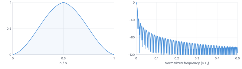
Bartlett-Hann hybrid. Balanced near/far sidelobe levels.[^ha1989] -36 dB sidelobe

lanczos(i, N)

$w(n) = \text{sinc}!\left(\frac{2n}{N-1} - 1\right)$

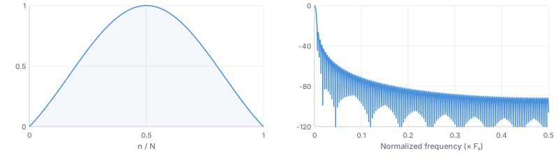
Sinc main lobe. Image resampling, interpolation (FFmpeg, ImageMagick).[^duchon1979] -26 dB sidelobe

parzen(i, N)

$w(n) = 1 - 6a^2(1-a)$ for $|a| \le 0.5$,   $w(n) = 2(1-a)^3$ for $|a| > 0.5$,   $a = |(2n-N+1)/(N-1)|$

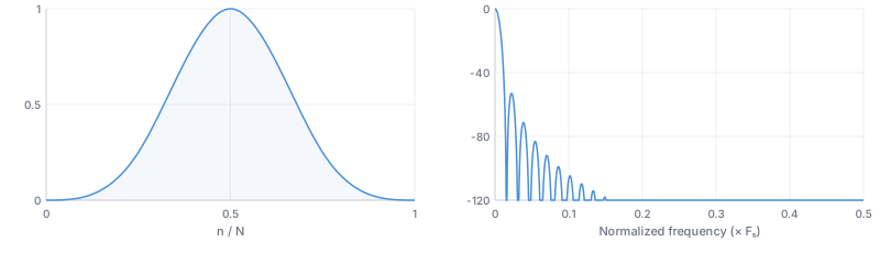
4th-order B-spline. Always-positive spectrum. Kernel density estimation.[^parzen1961] -53 dB sidelobe · -24 dB/oct rolloff

bohman(i, N)

$w(n) = (1-|a|)\cos(\pi|a|) + \frac{\sin(\pi|a|)}{\pi}$,   $a = \frac{2n-N+1}{N-1}$

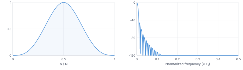
Autocorrelation of cosine window. Fast sidelobe decay, spectral estimation. -46 dB sidelobe · -24 dB/oct rolloff

Parameterized — adjustable tradeoff

kaiser(i, N, beta)

beta: shape — 0 = rectangular, 5.4 = Hamming, 8.6 (default) = Blackman.

$w(n) = \frac{I_0!\left(\beta\sqrt{1 - \left(\frac{2n-N+1}{N-1}\right)^2}\right)}{I_0(\beta)}$

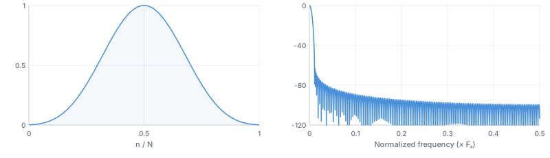
Near-optimal DPSS approximation via Bessel I₀. The standard parameterized window for FIR filter design.[^kaiser1974]

gaussian(i, N, sigma)

sigma: width, default 0.4.

$w(n) = \exp!\left[-\frac{1}{2}\left(\frac{2n-N+1}{\sigma(N-1)}\right)^2\right]$

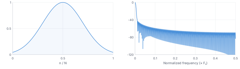
Gaussian bell, minimum time-bandwidth product. STFT/Gabor transform, frequency estimation via parabolic interpolation.[^gabor1946]

generalizedNormal(i, N, sigma, p)

sigma: width (default 0.4), p: shape — 2 = Gaussian, large = rectangular.

$w(n) = \exp!\left[-\frac{1}{2}\left|\frac{2n-N+1}{\sigma(N-1)}\right|^p\right]$

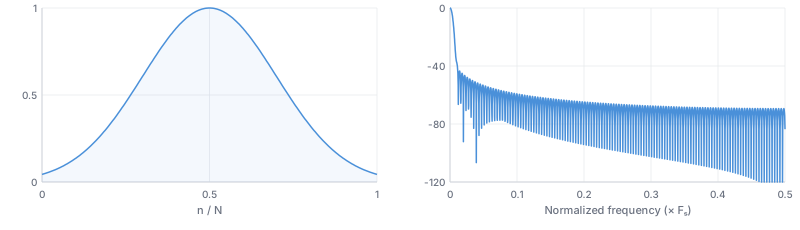
Continuous family between Gaussian and rectangular. Adjustable time-frequency tradeoff.

tukey(i, N, alpha)

alpha: taper fraction — 0 = rectangular, 0.5 (default), 1 = Hann.

$w(n) = \tfrac{1}{2}[1+\cos(\pi(n/(\alpha(N!-!1)/2)-1))]$ in tapered edges,   $w(n) = 1$ in flat center.

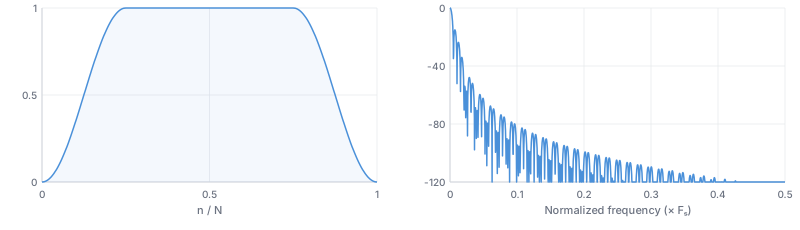
Flat center with cosine-tapered edges. Preserves signal amplitude while tapering. Vibration analysis, LIGO.

planckTaper(i, N, epsilon)

epsilon: taper fraction, default 0.1.

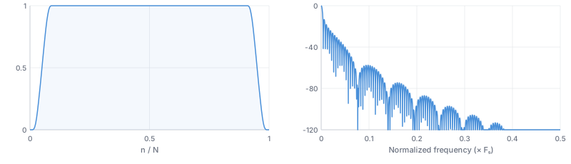
C∞-smooth bump function (infinitely differentiable). Gravitational wave analysis (LIGO/Virgo).[^mckechan2010]

powerOfSine(i, N, alpha)

alpha: exponent — 0 = rectangular, 1 = cosine, 2 (default) = Hann.

$w(n) = \sin^\alpha!\left(\frac{\pi n}{N-1}\right)$

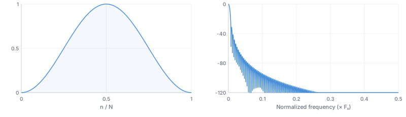
$\sin^\alpha$ family. Codec design, parameterized spectral analysis.

exponential(i, N, tau)

tau: time constant, default 1.

$w(n) = \exp!\left(\frac{-|2n-N+1|}{\tau(N-1)}\right)$

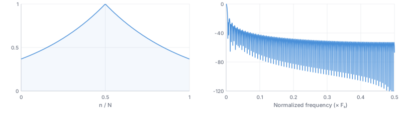
Exponential decay from center. Modal analysis, impact testing.[^harris1978]

hannPoisson(i, N, alpha)

alpha: decay, default 2. At α ≥ 2 the transform has no sidelobes.

$w(n) = \frac{1}{2}\left(1-\cos\frac{2\pi n}{N!-!1}\right)\exp!\left(\frac{-\alpha|2n!-!N!+!1|}{N-1}\right)$

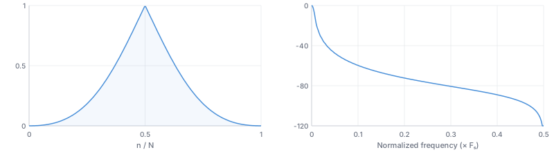
Hann × exponential. Unique no-sidelobe property enables frequency estimators using convex optimization.

cauchy(i, N, alpha)

alpha: width, default 3.

$w(n) = \frac{1}{1+\left(\frac{\alpha(2n-N+1)}{N-1}\right)^2}$

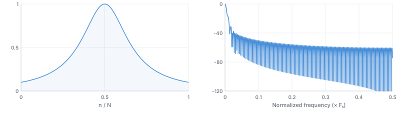
Lorentzian shape. Matches spectral line shapes in spectroscopy.[^harris1978]

rifeVincent(i, N, order)

order: 1 (default) = Hann, 2, 3. Throws for other values.

$w(n) = \frac{1}{Z}\sum_{k=0}^{K}(-1)^k a_k\cos\frac{2\pi kn}{N-1}$

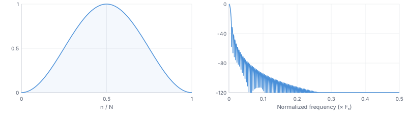
Class I cosine-sum optimized for sidelobe fall-off. Power grid harmonic analysis, interpolated DFT.[^rife1970]

confinedGaussian(i, N, sigmaT)

sigmaT: temporal width, default 0.1.

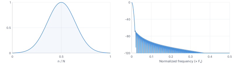
Optimal RMS time-frequency bandwidth. Time-frequency analysis, audio coding.[^starosielec2014]

Array-computed — cached

Compute the full window on first call, cache the result. Recomputed when parameters change.

dolphChebyshev(i, N, dB)

dB: sidelobe attenuation, default 100.

$W(k) = (-1)^k T_{N-1}!\left(\beta\cos\frac{\pi k}{N}\right)$,   $w = \text{IDFT}(W)$

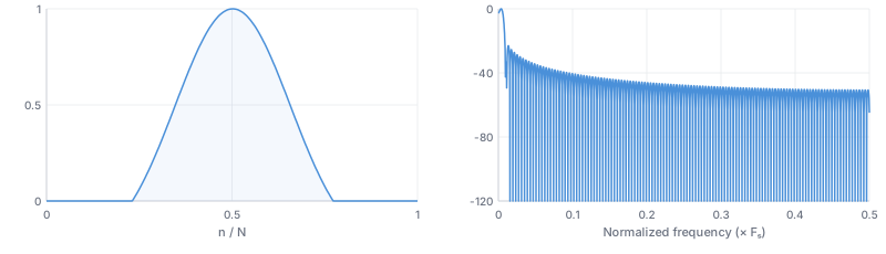
Optimal: narrowest main lobe for given equiripple sidelobe level. Antenna design, radar.[^dolph1946]

taylor(i, N, nbar, sll)

nbar: constant-level sidelobes (default 4), sll: level in dB (default 30).

$w(n) = 1 + 2\sum_{m=1}^{\bar{n}-1} F_m \cos\frac{2\pi m(n-(N!-!1)/2)}{N}$

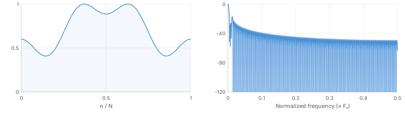
Monotonically decreasing sidelobes. The radar community standard for SAR image formation.[^taylor1955]

kaiserBesselDerived(i, N, beta)

beta: shape, default 8.6. N must be even.

$w(n) = \sqrt{\frac{\sum_{j=0}^{n} K(j)}{\sum_{j=0}^{N/2} K(j)}}$,   $K(j) = I_0!\left(\beta\sqrt{1-\left(\frac{2j-N/2}{N/2}\right)^2}\right)$

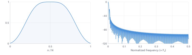
Princen-Bradley condition for perfect MDCT reconstruction. AAC, Vorbis, Opus audio codecs.[^princen1987]

dpss(i, N, W)

W: half-bandwidth [0, 0.5], default 0.1.

$\mathbf{T}\mathbf{v} = \lambda\mathbf{v}$,   $T_{jk} = \frac{\sin 2\pi W(j-k)}{\pi(j-k)}$

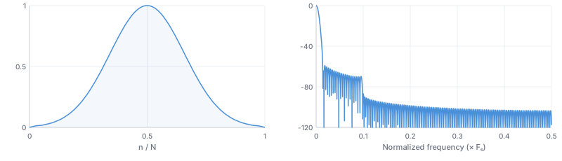
Dominant eigenvector of sinc Toeplitz matrix — provably optimal energy concentration. Also called Slepian window. Multitaper spectral estimation, neuroscience, climate science.[^slepian1978]

ultraspherical(i, N, mu, xmu)

mu: 0 = Dolph-Chebyshev, 1 (default) = Saramaki. xmu: sidelobe control (default 1).

$W(k) = C_n^\mu!\left(x_\mu\cos\frac{\pi k}{N}\right)$,   $w = \text{IDFT}(W)$

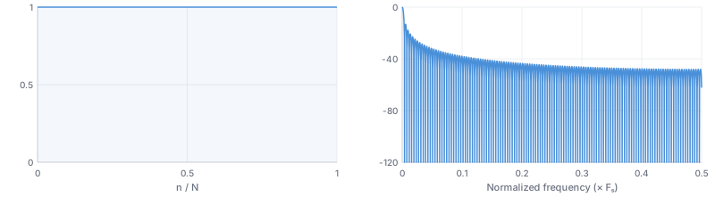
Gegenbauer polynomial window. Independent control of sidelobe level and taper rate. Antenna design, beamforming.[^streit1984]

Choosing a window

Every window trades frequency resolution (narrow main lobe), spectral leakage (low sidelobes), and amplitude accuracy (flat top). No single window wins all three.

Just get started hann — good all-round, zero edges, 50% COLADesign FIR filters kaiser or hamming — Kaiser is tunable, Hamming is the classicMeasure amplitudes accurately flatTop — < 0.01 dB scalloping lossHigh dynamic range (>80 dB) blackmanHarris — -92 dB equiripple sidelobesAudio codec (MDCT) kaiserBesselDerived or cosine — Princen-Bradley perfect reconstructionPreserve center, taper edges tukey — adjustable flat-top fractionRobust spectral estimation dpss — optimal for multitaper methodRadar / SAR taylor — monotonic sidelobes, radar standardAntenna array design dolphChebyshev or ultraspherical — optimal equiripple or tunable taperTune resolution/leakage continuously kaiser or gaussian — single-parameter adjustmentModal / impact analysis exponential — controlled decay for underdamped systemsFTIR spectroscopy connes — smooth apodization for interferogramsGravitational waves planckTaper — C∞ smooth, no spectral artifacts

Metrics

Three functions for quantitative window comparison:

import { hann, enbw, scallopLoss, cola } from 'window-function'

enbw(hann, 1024)                 // 1.5 — noise bandwidth (bins)
scallopLoss(hann, 1024)          // 1.42 — worst-case amplitude error (dB)
cola(hann, 1024, 512)            // 0 — perfect STFT reconstruction

• enbw(fn, N, ...params) — equivalent noise bandwidth in frequency bins. Rectangular = 1.0, Hann = 1.5, Blackman-Harris = 2.0. Lower = less noise.
• scallopLoss(fn, N, ...params) — worst-case amplitude error in dB between DFT bins. Rectangular = 3.92, Hann = 1.42, flat-top ≈ 0.
• cola(fn, N, hop, ...params) — COLA deviation. 0 = perfect STFT reconstruction at given hop size.

[^dolph1946]: C.L. Dolph, "A Current Distribution for Broadside Arrays," Proc. IRE 34, 1946. [^gabor1946]: D. Gabor, "Theory of Communication," J. IEE 93, 1946. [^bartlett1950]: M.S. Bartlett, "Periodogram Analysis and Continuous Spectra," Biometrika 37, 1950. [^taylor1955]: T.T. Taylor, "Design of Line-Source Antennas," IRE Trans. Antennas Propag. AP-4, 1955. [^blackman1958]: R.B. Blackman & J.W. Tukey, The Measurement of Power Spectra, Dover, 1958. [^connes1961]: J. Connes, "Recherches sur la spectroscopie par transformation de Fourier," Revue d'Optique 40, 1961. [^parzen1961]: E. Parzen, "Mathematical Considerations in the Estimation of Spectra," Technometrics 3, 1961. [^welch1967]: P.D. Welch, "The Use of FFT for Estimation of Power Spectra," IEEE Trans. Audio Electroacoustics AU-15, 1967. [^rife1970]: D.C. Rife & G.A. Vincent, "Use of the DFT in Measurement of Frequencies and Levels of Tones," Bell Syst. Tech. J. 49, 1970. [^kaiser1974]: J.F. Kaiser, "Nonrecursive Digital Filter Design Using the Sinh Window Function," IEEE Int. Symp. Circuits and Systems, 1974. [^hamming1977]: R.W. Hamming, Digital Filters, Prentice-Hall, 1977. [^harris1978]: F.J. Harris, "On the Use of Windows for Harmonic Analysis with the DFT," Proc. IEEE 66, 1978. [^slepian1978]: D. Slepian, "Prolate Spheroidal Wave Functions — V," Bell Syst. Tech. J. 57, 1978. [^duchon1979]: C.E. Duchon, "Lanczos Filtering in One and Two Dimensions," J. Applied Meteorology 18, 1979. [^nuttall1981]: A.H. Nuttall, "Some Windows with Very Good Sidelobe Behavior," IEEE Trans. ASSP 29, 1981. [^streit1984]: R.L. Streit, "A Two-Parameter Family of Weights for Nonrecursive Digital Filters and Antennas," IEEE Trans. ASSP 32, 1984. [^princen1987]: J.P. Princen, A.W. Johnson & A.B. Bradley, "Subband/Transform Coding Using Filter Bank Designs Based on TDAC," ICASSP, 1987. [^ha1989]: Y.H. Ha & J.A. Pearce, "A New Window and Comparison to Standard Windows," IEEE Trans. ASSP, 1989. [^heinzel2002]: G. Heinzel, A. Rudiger & R. Schilling, "Spectrum and Spectral Density Estimation by the DFT," Max Planck Institute, 2002. [^mckechan2010]: D.J.A. McKechan et al., "A Tapering Window for Time-Domain Templates," Class. Quantum Grav. 27, 2010. [^starosielec2014]: S. Starosielec & D. Hagemeier, "Discrete-Time Windows with Minimal RMS Bandwidth," Signal Processing 102, 2014.